1. Introduction to Energy-based models (EBMs)
Energy-based models (EBMs) are a class of probabilistic models that assign an energy to each configuration of the input data and learn to identify low-energy configurations. Unlike traditional supervised learning methods that directly predict output from input, EBMs instead use an energy function to determine stable configurations.
-
Key Concepts:
-
- Energy function: An energy function is a scalar function that maps input configurations to energy values. The goal is to find low-energy configurations, which correspond to stable states or patterns in the data.
-
- State: Each possible configuration of the model (e.g., the activations in a neural network) represents a state.
-
- Energy Minimisation: EBMs learn by finding the lowest-energy states, effectively discovering the most probable or stable states.
-
Why EBMs are relevant:
-
- They offer a flexible approach to model complex distributions without requiring explicit probability calculations.
-
- EBMs have foundational importance in unsupervised learning and associative memory and have influenced many modern architectures.
2. Core concepts of energy-based models
-
Energy functions: In physics, energy represents the system’s potential to perform work. In EBMs, energy functions encode how compatible a given state is with the underlying data distribution. Lower energy means the model is more confident in that state, making energy minimisation a core process.
-
Objective: The primary objective in EBMs is to minimise the energy of states that align with observed data, while pushing non-observed (or less probable) states to higher energies.
-
Connection to physics: EBMs are inspired by concepts from statistical mechanics, where systems evolve towards configurations that minimize free energy. This concept is leveraged to ensure the model “learns” representations by converging to stable, low-energy states.
3. Restricted Boltzmann Machines (RBMs)
3.1. Brief introduction to Restricted Boltzmann Machine
Restricted Boltzmann Machine (RBM) is a generative stochastic network that can learn a probability distribution over its training data.
3.2. Inference phase

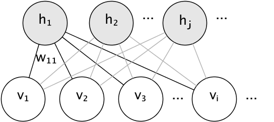
RBMs contain two layers: visible layer (\(v\)) and hidden (\(h\)).
In the scope of this blog, I will use Bernoulli RBM for better explanation. In the BernoulliRBM, all units are binary stochastic units. This means that the input data should either be binary, or real-valued between 0 and 1 signifying the probability that the visible unit would turn on or off.
The conditional probability distribution of each unit is given by the logistic sigmoid activation function of the input it receives:
\[\begin{split}P(v_i=1|\mathbf{h}) = \sigma(\sum_j w_{ij}h_j + b_i) \\
P(h_i=1|\mathbf{v}) = \sigma(\sum_i w_{ij}v_i + c_j)\end{split}\]
where \(\sigma\) is the logistic sigmoid function:
\[\sigma(x) = \frac{1}{1 + e^{-x}}\]
3.3. Training phase
The ultimate goal of RBM is to learn feature of the data (representation learning). In order to accomplish that, it uses a loss function to check whether the reconstructed data is close to the training data. If you work with today’s neural networks long enough, you may ask “Why shouldn’t we use L2, BCE, …”. However, at the time RBM was invented, these terminologies were not popular in the field. However, professor Hinton was inspired from energy in physics and decided to apply it, and that is how RBM was born.
Basically, energy is a measure of the system’s state that indicates how “stable” or “likely” that state is. In an RBM, the energy function assigns a lower energy to states that represent probable or stable configurations, and higher energy to unlikely or unstable configurations. For example, a cool water is stable and has low energy while boilingly hot water is unstable and has much higher energy (it can even power locomotives). In summary, we have to find the parameters that produce lowest energy in the training data and I will explain how it is done below.
Given a specific configuration of \(v\) and \(h\), we map it to the probability space.
\[p(v,h) = \frac{e^{-E(v,h)}}{Z}\]
The \(Z\) constant is a normalisation factor to ensure that we actually map to the probability space (based on Boltzmann distribution). Now let’s go to what we’re looking for; the probability of a set of visible neurons, in other words, the probability of our data.
\[p(v)=\sum_{h \in H}p(v,h)=\frac{\sum_{h \in H}e^{-E(v,h)}}{\sum_{v \in V}\sum_{h \in H}e^{-E(v,h)}}\]
To maximise likelihood, for every data point, we have to take a gradient step to make \(p(v) = 1\). The first thing we do is taking the log of \(p(v)\). We will be operating in the log probability space from now on in order to make the math feasible.
\[\log(p(v))=\log[\sum_{h \in H}e^{-E(v,h)}]-\log[\sum_{v \in V}\sum_{h \in H}e^{-E(v,h)}]\]
Let’s take the gradient with respect to the parameters in \(p(v)\).
\[\begin{align}
\frac{\partial \log(p(v))}{\partial \theta}=&
-\frac{1}{\sum_{h' \in H}e^{-E(v,h')}}\sum_{h' \in H}e^{-E(v,h')}\frac{\partial E(v,h')}{\partial \theta}\\ & + \frac{1}{\sum_{v' \in V}\sum_{h' \in H}e^{-E(v',h')}}\sum_{v' \in V}\sum_{h' \in H}e^{-E(v',h')}\frac{\partial E(v,h)}{\partial \theta}
\end{align}\]
Now I did this on paper and wrote the semi-final equation down as to not waste a lot of space on this site. I recommend you derive these equations yourself. Now I’ll write some equations down that will help out in continuing our derivation. Note that: \(Zp(v,h)=e^{-E(v,h')}\), \(p(v)=\sum_{h \in H}p(v,h)\), and that \(p(h \vert v) = \frac{p(v,h)}{p(h)}\).
\[\begin{align}
\frac{\partial log(p(v))}{\partial \theta}&=
-\frac{1}{p(v)}\sum_{h' \in H}p(v,h')\frac{\partial E(v,h')}{\partial \theta}+\sum_{v' \in V}\sum_{h' \in H}p(v',h')\frac{\partial E(v',h')}{\partial \theta}\\
\frac{\partial log(p(v))}{\partial \theta}&=
-\sum_{h' \in H}p(h'|v)\frac{\partial E(v,h')}{\partial \theta}+\sum_{v' \in V}\sum_{h' \in H}p(v',h')\frac{\partial E(v',h')}{\partial \theta}
\end{align}\]
After coming to equation (4), we still have a minor problem. Take a closer look at (4), we see that the second term of the equation requires simultaneous sampling of \(v'\) and \(h'\). In this scenario, we will use Gibbs sampling to overcome this (Check out a very intuitive explaination at Gibbs Sampling : Data Science Concepts).
4. Hopfield Network
4.1. Introduction to Hopfield network
Hopfield network, similarly, is another physics-inspired invention in this field. It also uses energy as a loss function for optimisation but have some differences in uses and the ways it works.
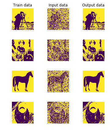
Hopfield is sometimes associated with content-addressable memory of human brains as it closely resembles them. For example, we usually have a rather vague image popped inside our head before we can fully retrieve the information in the brain. This evidence indicates that we ask our brain “Do you remember this blurry information and can get me a better, higher-quality version of it ?”. And Hopfield network does exactly that, you input a perturbed information and it will return more refined version of the input.

4.2. Inference phase

Updating one unit (node in the graph simulating the artificial neuron) in the Hopfield network is performed using the following rule:
\[s_i \leftarrow
\begin{cases}
+1 & \text{if } \sum_j w_{ij} s_j \geq \theta_i, \\
-1 & \text{otherwise}.
\end{cases}\]
where:
-
\(w_{ij}:\) is the strength of connection weight from unit j to unit i (the weight of the connection).
-
\(s_i:\) is the state of unit i.
-
\(\theta_i:\) is the threshold of unit i
Updates in the Hopfield network can be performed in two different ways:
-
Asynchronous: Only one unit is updated at a time. This unit can be picked at random, or a pre-defined order can be imposed from the beginning.
-
Synchronous: All units are updated at the same time. This requires a central clock
to the system in order to maintain synchronisation.
4.3. Training phase
Like RBM, Hopfield network also uses energy for optimisation.
\[E = -\frac{1}{2} \sum_{i,j}w_{ij}s_is_j - \sum_{i}\theta_i s_i\]
Usually, practitioners remove the $\theta$ for less computation by setting it to 0. And the energy becomes:
\[E = -\frac{1}{2} \sum_{i, j}w_{ij} s_i s_j\]
The energy here is the first order function, so taking derivative according to \(w_{ij}\) to find the optimal point is impractical. Therefore, we have to apply mathematical transformations to figure out.
\[-\frac{1}{2} \sum_{i, j}w_{ij} s_i s_j \ge -\frac{1}{2} \sum_{i, j} s^2_i s^2_j\]
\[<=> w^*_{ij} = \sum_{ij} s^2_i s^2_j \quad \text{(for 1 sample)}\]
\[<=> w^*_{ij} = \frac{1}{N} \sum_{n}^{N} \sum_{ij} s^2_i s^2_j \quad \text{for N samples}\]
5. Conclusion
In this post, I have walked you through the history and working of the two famous models that have laid the foundation for the rapid advancement of neural nets. As time progresses, better and more complicated models will be released, however, diving into how the basics work always help.
This is the end to the blog and I wish it could be useful to you. Peace out!
References
1. A Brain-Inpsired Algorithm For Memory - Youtube
2. Hopfield network - Wikipedia
3. Neural network models (unsupervised)
4. Intuition Behind Restricted Boltzmann Machine (RBM)